Lab 6:  Steady-State Frequency Response of an RC Network

In this lab you will use the function generator and the oscilloscope to measure the voltage and phase (as a function of frequency) in a series RC network. If we connect the RC network to an AC supply, such as a function generator, a steady-state current will flow. The series RC network functions as a frequency dependent voltage divider. In this lab we will observe the magnitude and phase of the voltages across R and C as functions of frequency.

Reading:  2.20.7-8, 7.4, 9.0-3

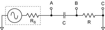
The RC network. Construct a series RC circuit as shown above using a 10 K resistor and a 0.01 μF capacitor. Calculate the 3dB frequency you expect based on the labeled component values and record it in your notebook. Now measure the resistor using your DMM and record it in your notebook. Measure the capacitance of your capacitor with the capacitance meter and record that in your notebook. Later you will model the circuit using these values.

Set up. Connect the function generator to your circuit as shown above. Use a BNC Tee to also connect the function generator to channel 2 of your scope. Set the function generator to output a 1 kHz sine wave with a 5 Vp-p amplitude and zero DC offset. Trigger the scope from channel 2.

Explore the Sweep options in the trigger menu. Sweep = Normal only acquires and displays a sweep when a trigger event occurs. Sweep = Auto acquires and displays a sweep even if no trigger event has occurred within some preset time. Sweep = Single acquires an displays a single sweep and is controlled with the Run/Stop button

Oscilloscope probes. Obtain a scope probe and connect it to channel 1.

This paragraph is repeated from an earlier lab for your convenience. If you are unfamiliar with scope probes, your instructor will help you. Scope probes come in two common flavors, 1X and 10X. The 10X probe divides the voltage by a factor of ten. The 1X probe does not change the voltage. Most of the probes in the lab have a switch to change flavors. Check to see if yours has a switch. Test your probe by touching it to the test port of the scope. The test port has a 1 kHz 3.0 Vp-p voltage for testing your probe. What variety of probe do you have? Is it a 1X or 10X? Can it be switched? Is your probe functioning correctly? Check the CH1 menu, which probe is selected? It does not matter which flavor you have as long as you know which it is.

In this lab you will use the 1X setting of the probe on channel 1.
Configure channel 1 for the 1X probe. CH1 menu: probe = 1X.

 

Additionally you must select DC coupling for both channels.
CH1 menu: coupling = DC and CH2 menu: coupling = DC

 

Using AC coupling will mess up your results for this lab!

DC coupling is always the safest setting.

In general, only use AC coupling if you have a very good reason.

Plan your measurements. We want to measure the magnitude and the phase of the voltage across the resistor V_R and across the capacitor V_C. We need to measure the response over many orders of magnitude of frequency (1 Hz to 3 MHz). Clearly we need to take data points at a minimum of ~1 Hz apart at low frequencies. However maintaining a constant (1 Hz) separation between data points is impractical. To do so would require more than 10⁶ points to span the range of frequencies of interest. It is often the case in physics and engineering that a physical system has a behavior that is naturally characterized by geometric step in frequency. A geometric progression is characterized by a constant ratio between adjacent points. This is convenient because the points have a uniform separation when plotted on a log scale. This naturally gives us the fine resolution we need at low frequency and the courser resolution at high frequency. For example 1, 2, 4, 8, 16, ... and 10⁰, 10¹, 10², 10³, ... are both geometric progressions. The latter progression is commonly described as 1 point per decade. A common progression that gives 2 points per decade is 10⁰, 10^0.5, 10¹, 10^1.5, .... This can be approximated as 1, 3, 10, 30, .... Note that 10^0.5 ≈ 3. This is a useful approximation for experimental measurements because it is often not important exactly what the value of the frequency as long as we measure that frequency. The design of the data collection is simply to spread the data points across frequency in a way that best characterizes the system’s response while minimizing the number of data points.

For this lab we will record two points per decade (as per the sample table).

All measurements will be made using the scope. You have seen in previous labs that the numbers on the function generator and on the scope do not agree. So we will make all the measurements using one device, your scope.

Measuring frequency. We will measure the period, because the period is used for calculating the phase. Frequency will be calculated form the period during data analysis. You will need to do this for each frequency you use.

Measuring phase. Phase is always a relative measurement. That is, it is measured with respect to some reference point. In this measurement we are comparing the phase shift of the sine wave V_R or V_C with respect to V₀. Thus V₀ is the phase reference. Measuring the time difference between a reference point on the V₀ sine wave and the same point on the V_R or V_C sine waves best does this.

The phase shift in degrees is then obtained knowing the period of the wave and that a single period is 360 degrees.

Scope set up. You will use a combination of automatic and cursor measurements.

Automatic measurement set up.

·         Clear any existing measurements.

·         1^st measurement:  source = CH1; Voltage = Vp-p

·         2^nd measurement: source = CH2; Time = Period

·         3^rd measurement: source = CH2; Voltage = Vp-p

Cursor set up.

·         Mode = Track

·         Cursor A = CH2

·         Cursor B = CH1

The time delay of channel 1 with respect to channel 2 is now Δx.

Make the measurements V_R and V_C. Set up the trace V_R and V₀ on the scope so that you can observe one complete cycle. For each frequency your will need six measurements: The period and the magnitude of the signal applied to the network (channel 2), the magnitude of the voltage on V_R and V_C, and the time delay (phase shift) of V_R and V_C with respect to V₀. Prepare a table in your notebook to record these values.

Record the amplitude & time—your raw data. You will use this data to calculate frequency, phase, etc. in your analysis spreadsheet.

Note that some of the data will be very noisy at low amplitudes. The automatic measurement will not work so you will need to do it manually.

Sample table. Create a table like this in your lab notebook. You will enter it into a spread sheet later to calculate frequency, phase, V_C/V₀, and V_R/V₀.

Instruction for the data work up will be given in the second lab period.

Data work up. Use excel to make the following graphs. Your graphs must have their axes labeled and properly scaled in the appropriate units.

Excel table.

Enter the data table from the previous page into your laboratory notebook. in the same format as above. Now add additional columns so that you can work up you data.

 

First the voltage magnitude.

1) Plot V_R/V₀ in dB vs log frequency. Your plot should consist of two linear regions (a horizontal and a sloped region) and a transition region in between.

2) Plot V_C/V₀ in dB vs log frequency. Your plot should consist of two linear regions (a horizontal and a sloped region) and a transition region in between.

3) Plot V_R/V₀ in dB vs log frequency w/ best fit slope. Perform linear regression on the sloped portion of your line. ONLY USE THE POINTS BELOW −10dB for your fit. Your slope should be close to +20. Using the slope and intercept you obtained from the regression, plot the best fit line for this section between 0 and about −60 dB.

4) Plot V_C/V₀ in dB vs log frequency w/ best fit slope. Perform linear regression on the sloped portion of your line. ONLY USE THE POINTS BELOW −10dB for your fit. Your slope should be close to −20. Using the slope and intercept you obtained from the regression, plot the best fit line for this section between 0 and about −60 dB.

5) Calculate the frequency of the 3dB points from your-best fit lines. The x intercepts of the sloped part of your lines intercept the x axis at the 3dB frequency. Calculate the x intercepts for the two best-fit lines. Average these log f values to obtain log f_3dB. Calculate f_3dB and from this.

6) Model you data and plot it with your experimental data. Make two plots, (V_R/V₀) in dB vs log frequency and (V_C/V₀) in dB vs log frequency. Use open symbols for you experimental data and a solid line for your model. Modeling means to calculate (predict) the behavior you expect to observe. You measured R in the lab. If your were not able to measure C, simply use the nominal value printed on the capacitor. Model your circuit using these values. First work out the algebraic solutions for V_R/V₀ and V_C/V₀ (these will be functions of frequency). Then calculate V_R/V₀ and V_C/V₀. as a function of frequency. Because these are values you calculate, it is easy to calculate and to plot a finer mesh than you measured. Do your calculations using a 10 point per decade or finer geometric progression.^* Plot your model results by connecting the points with lines. Do not use symbols on the model data points. Also plot on the same graph your experimental data. Plot your experimental data as open symbols, but do not connect them with lines. This is common experimental practice and will show how well you measurements fit the theoretical model. What is the frequency at the −3dB point (V/V₀ = 1/√2) you measure experimentally? What is predicted by the model? What is the slope of the line in the sloped region?

Now plot the phase information.

7) Plot θ_R (degrees) vs log frequency.

8) Plot θ_C (degrees) vs log frequency.

10) Model you data and plot it with your experimental data. Make two plots, θ_R vs log frequency and θ_C vs log frequency. First work out the algebraic solution for θ_R and θ_C (these will be functions of frequency). Then calculate θ_R and θ_C as a function of frequency. Now plot them as your were instructed to do for V_R/V₀ and V_C/V₀ in part 6 above. What is the phase at the 3dB frequency (V/V₀ = 1/√2) you measured experimentally? What is predicted by the equation? What phases do you expect at the limiting frequencies f → 0? and f → ∞? How close do you measurements approach to these values?

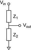
11) Consider the series RC network as a filter. Draw the schematic for the high pass configuration and for the low pass configuration. The following figure is a guide. You will need to replace the general impedances with the R and the C.

12) You measured V_R and V_C versus frequency. Which data sets correspond to a high-pass filter and which to a low-pass filter?

*Notes on generating a log progression for your model circuit:  One way to generate a geometric progression begins with an index. In this example the index n runs from 0 to 65. The points per decade is p = 10. The equation f = 10^(n/p) will generate a geometric progression 10 points per decade running from 10^0 to 10^6.5 (1 Hz – 3 MHz).

Lab Report Check List
Steady State RC Network

0)   Coversheet w/ name of this lab, your name, your lab partner’s name, & your section.

A)  5pts      Part 0.        Print of your Excel data table. (Not the model calculations!!!)

B)  10pts    Parts 1/2.   Graph with your V_R and V_C data:  V_R/V₀ in dB vs log frequency and V_C/V₀ in dB vs log frequency. You can put both data sets in the same graph as long as each data set is clearly labeled.

C)  10pts    Parts 3/4.   Graph of V_R and V_C data with the best fit slopes:

D)  5pts      Parts 3/ 4.  Print of the regression sheets. OR trendline graphs with the equations.

E)  10pts    Part 5.        The f_3dB measured from your linear regression. Show your work, starting from the regression slopes and intercepts.

F)   15pts    Part 6.        Graph of V_R and V_C data with your model.

G)  10pts    Parts 7/8.   Graph with your θ_R and θ_C data:  θ_R (degrees) vs log frequency and θ_C (degrees) vs log frequency.

H)  15pts    Part 10.      Graph of θ_R and θ_C data with your model.

I)   5pts      Part 10.      Answer questions in part 10.

J)   5pts      Part 11.      Answer questions in part 11.

K)  5pts      Part 12.      Answer questions in part 12.

L)  5pts.     Make a table of the values for f_3dB. It should include:

1) the value you calculate from the nominal value of R and C (By nominal value, I mean the value printed on the component.),

2) the value you found when making your measurements, and

3) the value you determined in part 5.

Report the value of R that you measured. Using your measured value of R, calculate the C from the your two experimental f3dB measurements and include this as a column in the table.

M) Lab Notebook pages

 

Each graph must have the following components:

• The correct quantities plotted and on the correct axes.
• A main title.
• Both axes must have titles with w/ units.
• Both axes must have tick marks and labels.
• The experimental data are typically plotted as symbols.
• The best fit line obtained by linear regression is plotted as a line.
• Use a legend to identify symbols and lines when the graph contains more than one data set.

Graphs that to not fulfill these basic requirements will not be accepted.