Lab
5: Transient Response of an RC Network:
measuring the time constant
In this lab you will use the function generator and the oscilloscope to measure
the transient voltages in a series RC network. If we connected the RC network
to a DC supply, such as a battery, a transient current will flow as the
capacitor charged. This current dies off exponentially with the time constant
RC. In this lab we will observe these transients by applying a DC voltage that
periodically changes polarity. The charging transients can then be observed
each time the polarity flips.
This lab is more formal than you previous labs. It requires some writing, data analysis, graphing, and linear regression. When you answer the questions in the lab, short answers are not sufficient.
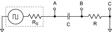
Overview: The RC network. Construct a series RC circuit as shown above using a 10 K resistor and a 0.01 μF capacitor. Calculate the RC time constant you expect based on the labeled component values. Now measure the resistor using your DMM and record it in your notebook. After we measure the RC time constant of your circuit we will be able to calculate the actual capacitance.
A) Oscilloscope probes. Obtain a scope probe and connect it to channel 1. If you are unfamiliar with scope probes, your instructor will help you. Scope probes come in two common flavors, 1X and 10X. The 10X probe divides the voltage by a factor of ten. The 1X probe does not change the voltage. Most of the probes in the lab have a switch to change flavors. Check to see if yours has a switch. Test your probe by touching it to the test port of the scope. The test port has a 1 kHz 3.0 Vp-p voltage for testing your probe. What variety of probe do you have? Is it a 1X or 10X? Can it be switched? Is your probe functioning correctly? It does not matter which flavor you have as long as you know which it is.
In this lab
you will use the 10X setting of the probe on channel 1.
Configure channel 1 for the 10X probe. CH1 menu: probe = 10X.
B) Function generator set up. Connect the function generator to your circuit as shown above. Use a BNC Tee to also connect the function generator to channel 2 of your scope. Set the function generator to output a 500 Hz square wave with a 5 Vp-p amplitude and zero DC offset.
C) Scope set up. Set up the scope so you can see the traces of both channels. Connect the probe to A and the ground to C. Verify that this voltage is and should be the same as observed in channel 2. Disconnect the probe ground from C. Does it make a difference? Why/Why not?
D) Set up and plan your measurements. We want to measure the voltage across the resistor Vr and across the capacitor Vc. Before we take detailed measurements, let’s first survey the situation to plan how this is to be done. Connect the probe to B to measure the voltage across the resistor. However if we connect the probe to A, we only measure the total voltage across R and C. Connecting the probe ground to B removes R from the network. Come up with a simple method to measure Vc and verify that it works. If you are unsure, ask your instructor before proceeding. (Hint: recall the grounding issues you encountered in the AC Test Instruments lab.)
E) Make the measurements Vr and Vc. Set up the scope for the measurements.
- Triggering. rising edge from channel 2 (the square wave).
- Horizontal scale. 100 μs/div. Center the zero.*
- Channel 1 vertical scale, 100 mV/div. Adjust the position so you can see the start of the transient.
- Channel 2 vertical scale, 1 V/div. Center the zero.*
- Set up the measurement. Cursor mode = track, cursorA = CH1, cursorB = NONE
Start with Vr. Position the cursor for the start of the transient. You have expanded the scale (200 mV/div rather than 1 V/div) to get accurate measurements. You will need to use the vertical position adjustment to bring the start of the transient into the display area. Record the voltage at 0.0, and 4.0 μs. Then every 40 μs. (viz. 40, 80, 120, … μs) until you reach the end of the transient (1000 μs). As you move the cursor along the trace, you will need to adjust the vertical and horizontal position to keep the cursor on the display. Once the channel 1 zero volts level becomes visible, you need to start increasing the sensitivity (V/div) of channel 1 to further expand the wave. You should finish at 5 mV/div. Record these points in your notebook. You will analyze them later. Now using the same scope set up, measure the Vc. Record the voltage at the SAME time points you used for Vr.
F) Data work up. Use excel or another plotting program. Your graphs must have their axes labeled and properly scaled in the appropriate units.
1) Plot Vr vs time
2) Plot Vc vs time.
3) Plot (Vr+Vc) vs time. Do the voltages sum to the total voltage applied across the series network? Should they? Why?
4) Plot log(Vr) vs time. Fit the good part of your data to a straight line. We know that Vr(t) = Vr(0)exp(–t/RC). In your lab report, start with this equation to show that the slope of the line should be –1/RC. From linear regression of your line, what is the RC time constant of your circuit? (with correct units!)
5) You measured R with your DMM. Calculate C from you measurement of the RC time constant.
In your lab report be sure to include all of the schematics, derivations of the equations, all of the calculations, and plots. Use significant figures for error propagation. Explicitly answer all the questions posed in the lab.
*A quick way to center the zero
is to press and hold the position knob.
Sample table. Create a table like this in your lab notebook.
|
measurement |
time (s) |
VR (volts) |
VC (volts) |
||
|
DO NOT RECORD PLEASE USE YOUR |
|
|
|
||
|
|
|
|
|
||
|
|
|
|
|
Lab
Report Check List
Time Constant of an RC Network
0) Coversheet w/ name of this lab, your name, your lab partner’s name, & your section.
1) 2pts. What type of probe did you use? (section B)
2) 5pts. Discuss and explain your observations on grounding from section C.
3) 5pts. Answer questions in F.3.
4) 5pts. Show that slope is –1/RC (F.4)
5) 10pts. Print of data table from excel.
6) 15pts. Plot of Vr vs t (F.1)
7) 15pts. Plot of Vc vs t (F.2)
8) 15pts. Plot of Vr+Vc vs t (F.3)
9) 5pts. Print of ln(Vr) vs t regression data from excel. Or the print of the ln(Vr) vs t graph with the trend line showing the equation with slope and intercept. (F.4)
10) 15pts. Plot of ln(Vr) vs t with ALL experimental points and best fit line using slope & intercept from linear regression. (F.4)
11) 4pts. The time constant of your circuit (F.4)
12) 4pts. Calculation of
C from your slope.
Show units and substitution into your equation. (F.5)
13) Lab Notebook pages
Scientific Graphing. We often describe of a graph as a plot of A versus B. This means that A is plotted on the y axis and that B is plotted on the x axis. Generally the quantity plotted on the y axis is also the dependent variable and that on the x axis is the independent variable—that the value of A is dependent on B. Thus in the experiment we would vary B and then measure A as a function of B.
The following example is a graph of count rate versus time.
 |
A graph has a main title which describes what it is a graph of. In this example it is a graph of “Count Rate Versus Time”. Each axis also has a title which describes what is plotted on that axis AND the units of the quantities on the labels. In this example the y axis is “Count Rate” in units of “s−1”. The x axis is “Time” in units of “s”. Tick marks on the axes show uniform intervals. The tick marks are labeled with the values. The data points are plotted on the graph as symbols. In this example the data points are represented by open circles. The value corresponding to the data is in the center of the symbol. The line that best fits the experimental data is also plotted on the same graph with the symbols so that the correlation and scatter of the experimental data point can be easily seen.
Each graph must have the following components:
- The correct quantities plotted and on the correct axes.
- A main title.
- Both axes must have titles with w/ units.
- Both axes must have tick marks and labels.
- The data are plotted as symbols.
- The best fit line obtained by linear regression is plotted as a line.
Graphs that to not fulfill these basic requirements will not be accepted.
